Chapter 10 - Text Mining

Authors: Alon Bartal, Avi Ma’ayan, Giacomo Marino

Maintainers: Giacomo Marino

Version: 0.1

License: CC-BY-NC-SA 4.0

---

The objectives:

• Describe basic concepts and methods in text mining

• Exploit information contained in textual documents for data analysis to uncover interesting patterns.

• Conceptually understand the mechanism of advanced text mining algorithms, text classification and clustering, and their applications in biomedical problems.

• Understand how to choose appropriate models for text analysis tasks.

Textual Data

Data be can structured (e.g. tables), semi-structured (e.g. emails, XML), or unstructued (e.g. plain text).

Text data grows dramatically from sources such as Twitter, emails, blogs where users create and share content.

Biomedical Textual Data

There is also an explosive growth of biomedical literature (Zhang et al 2019; Westergaard et al. 2018). In the scientific community, researchers cannot read or get insights quickly from these large textual datasets. Exposure to innovative information is important to develop breakthroughs. Therefore, doctors, practitioners, and scientists need to be updated with recent findings. For example, detecting side effects of drug-drug combinations.

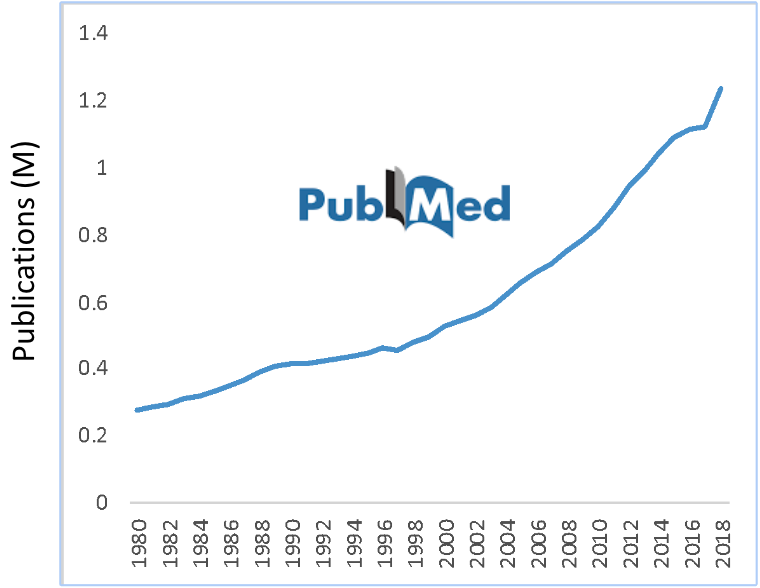
Fig. 10 Data volume is doubling every two years ~ 79% is text. Sourced from: https://www.nlm.nih.gov/bsd/licensee/baselinestats.html

Automatic Discovery of Information from Textual Data

This can be separated into three main parts:

• Text retrieval

• Information extraction

• Data mining: exploring relations among extracted pieces of information

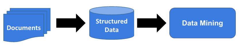
Fig. 11 Pipeline for automatic discovery of information from textual data.

Natural Language

Natural langues are those that humans use to communicate through both textual (e.g. tweets, emails, SMS) and verbal (e.g. Skype, phone calls, class). Natural language processing (NLP) is so that computers may understand human language. This could include tasks such as:

• Text classification

• Sentiment analysis

• Named entity recognition (NER)

Fig. 12 Example of text on which NLP might be used. The highlighted green piece of text might reflect a positive sentiment, while the red might reglect negative sentiment.

The Figure about highlights an amazon review which could be analyzed in terms of sentiment analysis. An Amazon merchant may, for example, want to analyze the sentiment of the reviews for a competive product to gain more insight than simply the star rating average. In the example above groups of words may contribute to the postive or negative sentiment of the reivew and some examples are highlighted in the relevant color.

Natural Language Processing

Natural Language denotes a complex communication system that is natrually occurring and evolving. Thus, it is not the same as well-defined formal language such as HTML or Python. The processing of this is a computational “understanding” of a natural language such as English, American Sign Language (ASL), or Spanish.

Text Representation

The represenation of text is broken down into smaller components which include:

• Numbers (all data is represented as numbers at a low level)

• Characters (e.g. ASCII)

• Words (e.g. stop words, stemming, lemmatization).

  • Tokenization: split text into individual words

    • Identify stop words (e.g. “the”, “a”, “and”)

• Vectors (e.g. each word can be represented as a vector)

  • TF-IDF (term frequency - inverse document frequency)

  • Word2Vec

  • BERT

Some possible tasks that could be done using NLP models:

• Dectecting topics in a coripus of documents

  • E.g., collect all documents about the same topic from PubMed

• Named Entity Recognition

  • Dectecting gene names in articles

• Semantic analysis

  • Detecting the mood of a person who wrote the post

  • Recommending content based on mood (e.g. music)

• Documents classification

  • Detecting the number of topics in a corpus and classifying documents by topic

Language Models

In language models, a context is the history of a word, i.e., previous words. Recent models define the context of a word by both sides of a word (before and after a word). Language models are built on the fact that words often come in a specific order - the goal is to capture a language structure based on word statistics. In addition, different domains contain different word statistics and sequences, as well as different use in upper/lower case. Given a context, a language model predicts the probability of a word occurring in that context, but what window side is sufficient to capture the context of a word?

Context of a word

• The history of a word, i.e., previous words

  • Recent models use context to both sides of a word

  • Words often come in a specific order

• What about the knowledge domain? Upper/lower case? The language/ - For now we ignore it

The Markov assumption

• No need for full history of a word (only need ~ 2-5 words)

• N-Gram models

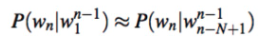
N-gram

N-gram finds the probability of a word given its previous words. Here we capture a language structure based on word statistics and predict of the occurrence of a word based on the occurence of its \(N - 1\) previous words.

• Bigram (\( N = 2 \)) model predicts the occurence given 1 previous word

• Trigram (\( N = 3 \)) model predicts the occurence given the 2 previous words

So given tha text coupus and \(WORD_i\) &rarr the probability of of \(WORD_j\) is:

• Using the Bayseian rule:

Consider the following example:

1. “Text mining is fun.”

2. “I love Text mining for biology.”

3. “I wish we would study Text classification.”

What is the probability of the word “mining” following the word “Text”?

What is the probability of the word “classifcation” following the word “Text”?

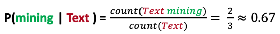
So, if a user wanted to predict the word after “Text” which word would our model produce?

Training N-gram Model

Given a corpus of documents (e.g. 1M PubMed articles), we might for example use 70% for training and reserve 30% percent for testing.

How might we handle a word that is in the testing set but was never seen in the training set (OOV - out of vocabulary)?

• W = Union of words in Training documents

The solution is to use Add-one (Laplace smoothing)

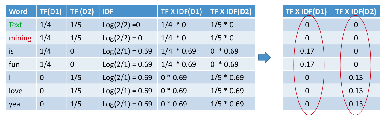
Term Frequency X Inverse Document Frequency (TF-IDF)

Given a set of documents, words that are more frequent in one document and are less frequent in all other documents are important.

• Term frequency (TF) - Number (n) of times a \(word_i\) occurs within a \(document_j\) compared to the total number of words (k) in that document

  • \( tf_{ij} = \frac{n_{ij}}{\sum_{k} n_{ij}} \)

• Document frequency - Number of times a word occurs within all documents divided by the number of documents containing the word

• Inverse Document Frequency:

  • \( idf(w_i) = log(\frac{|\text{Documents}|}{|\text{Documents containing }w_i|})\)

Combining these two formulas:

• \(TF*IDF(w) = tf_{ij}*log(\frac{|\text{Documents}|}{|\text{Documents containing }w_i|})\)

TF-IDF Example

Text can contain special characters and unwanted spaces. Depending on the task, we might want to remove special characters and numbers.

Consider the following example:

• D1: “Text mining is fun”

• D2: “I love Text mining yea”

Common words are zero (non significant)

Here’s a solution in Python to the above example:

# import libraries
import numpy as np
import re
import nltk
from sklearn.datasets import load_files
nltk.download('stopwords')
import pickle
from nltk.corpus import stopwords

# create text documents
D1 = "Text mining is fun"
D2= "I love Text mining yea"

# Tokenize
BOW_D1 = D1.split(' ')
BOW_D2 = D2.split(' ')

# Get all words in the corpus
dic = set(BOW_D1).union(set(BOW_D2))

# create a vector with zeros for doc D1
word_count_D1 = dict.fromkeys(dic, 0)
# count word frequency in D1
for word in BOW_D1: 
    word_count_D1[word] += 1

# create a vector with zeros for doc D2
word_count_D2 = dict.fromkeys(dic,0) 
# count word frequency in D1
for word in BOW_D2:
    word_count_D2[word] += 1

def TF(word_count, BOW):
  k = len(BOW) # number of words in a document
  tfDict = {}
  for word, count in word_count.items():
      tfDict[word] = count / float(k)
  return tfDict

tf_D1 = TF(word_count_D1, BOW_D1)
tf_D2 = TF(word_count_D2, BOW_D2)

import math
def IDF(documents):
  N = len(documents)
  idfDict = dict.fromkeys(documents[0].keys(), 0) # create a vector with zeros
  for document in documents:
      for word, val in document.items():
          if val > 0:
              idfDict[word] += 1
  
  for word, val in idfDict.items():
      idfDict[word] = math.log(N / float(val))
  return idfDict

idfs = IDF([word_count_D1, word_count_D2])

def TFIDF(tfBagOfWords, idfs):
    tfidf = {}
    for word, val in tfBagOfWords.items():
        tfidf[word] = val * idfs[word]
    return tfidf

# compute TF-IDF values for the documents
import pandas as pd
tfidf_D1 = TFIDF(tf_D1, idfs)
tfidf_D2 = TFIDF(tf_D2, idfs)
df = pd.DataFrame([tfidf_D1, tfidf_D2])

NLP Models for Word Embeddings

Recent models uses word embeddings. The main idea is to represent a word by its neighbors. Embeddings are vectors generated to represent each word i.e. embeddings since computers can only analyze numbers and do not understand the raw text.

Word2vec and GloVe are word embedding models that use a two-layer neural network (1 hidden layer) where the inputs are words and the output are words in a vector space. Words with common contexts are located closer in the vector space. These models proved useful in capturing semantic relations between words. Figure 2 presents a two-dimensional vector representation of the words Queen, King, Woman, and Man based on a Word2Vec model.

• Word2vec (Milkolov et al. 2013), GloVe (Pennington et al. 2014)

  • Two-layer neural network (1 hidden layer)

  • Input: words

  • Output: words in a vector space

  • Words with common contexts &rarr closer in the vector space

  • Capture sematic relations

• Similar application gene2vec - the likelihood that genes will co-occur

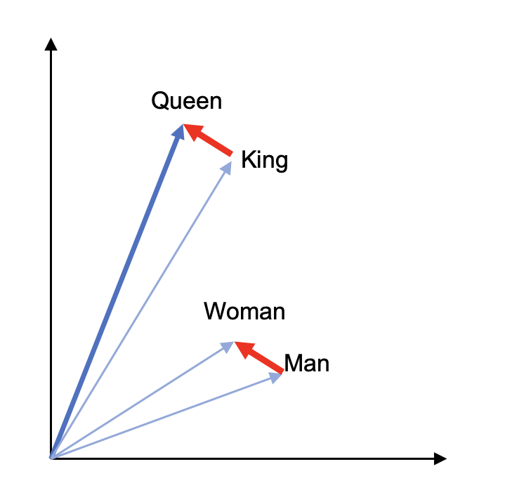
In figure above we can mathematically represent the vector of the word Woman by a linear combination of other words: v(king)-v(man)+v(woman) = v(queen).

Word2Vec

Word2Vec is like an autoencoder, encoding each word in a vector. However, the difference is that we train words against neighboring words in the input corpus in order to learn the context of a word.

How is the context of a word learned?

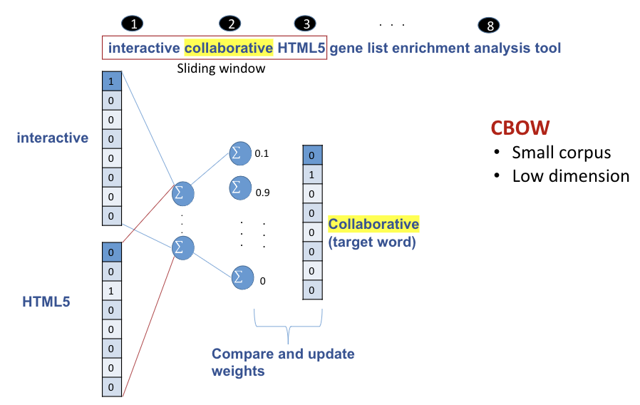
• Continous Bag-of-Words (CBOW)

  • Predicts target words from the surrounding (window size) (context words)

• Skip-Gram

  • Predicts surrounding (window size n~5) context words from the target words (inverse of CBOW) and treats each context-target pair as a new observation.

  • Given a word create word pairs (from its n-grams)

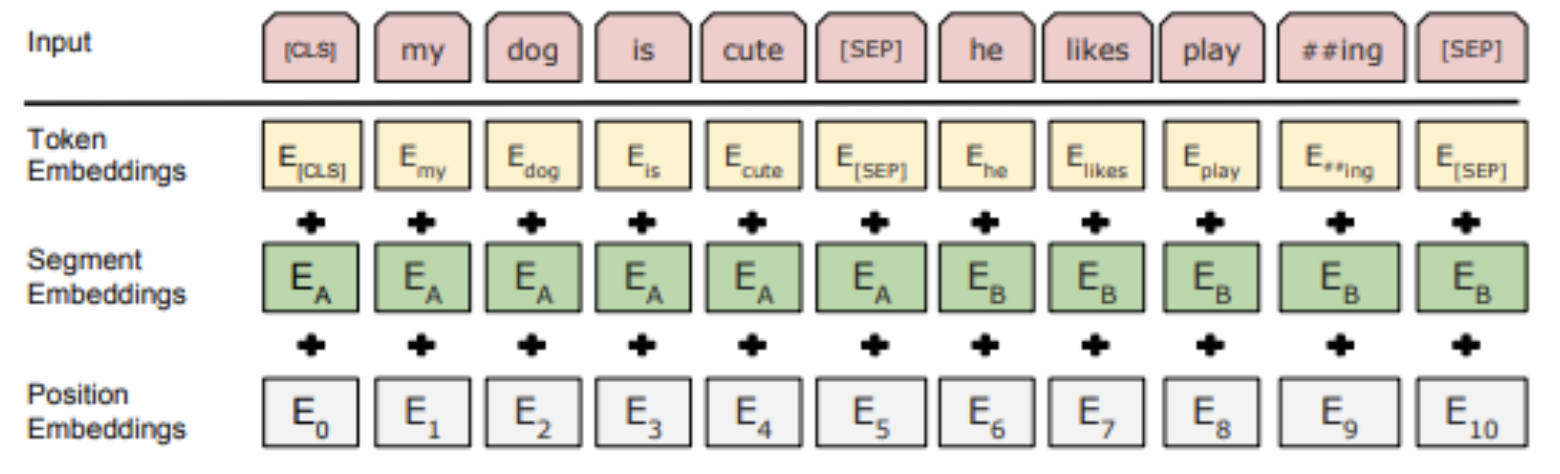
Fig. 13 CBOW and Skip-Gram methods for training a Word2Vec model.

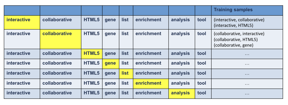
Skip-Gram

Consider the following example:

• “interactive and collaborative HTML5 gene list enrichment tool”

  • Delete stop words

  • Window size: 2

Training

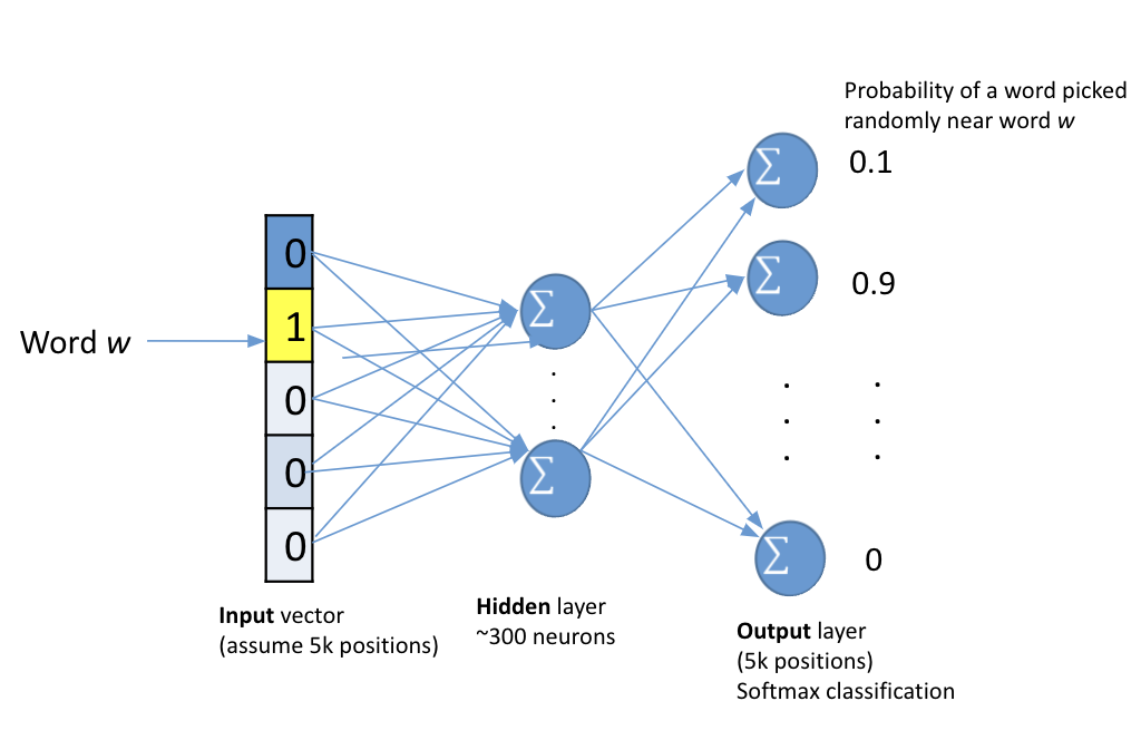
• Train a neural network with a single hidden layer

  • Use hidden weights of trained network as word embeddings

• How to feed a word into a neural network?

  • Create a vector of the same length as the volcabulary.

    • All zeros

    • The index that represents the word is assigned “1”

• If the word vector does not accurately predict that word’s context, the componets of the vector are adjusted. The following figures represent this process. Neural networks are covered in more depth in Chapter 16: Intro to Machine Learning.

Consider the following example from the sentence we considered before:

Gene2vec is a biological extension of Word2Vec that uses gene connectivity as proximity to infer the likelihood that genes will co-occur (i.e. interact). A limitation with Word2Vec is that it ignores the internal structure of words by considering only one direction of the words (instead of both directions - before and after). Another limitation is by allowing only one vector per word which can incorporate double meaning in a single vector. For example, a word can have different meanings 1) “Go there…”, and 2) “Let’s play Go”. Therefore, Word2Vec can yield unsatisfactory results when applied to biomedical text since biomedical word distribution differs from other corpora (Lee et al. 2019; Zhang et al. 2019) Recently several solutions have been suggested that use recurrent neural networks (RNN) which are slow, hard to parallelize, and hard to gain access to many steps back. The long short-term memory networks (LSTMs) which are also slow, use only one direction. Some models are bidirectional and account for the structure of words, e.g., Bidirectional Encoder Representations from Transformers (BERT) (Devlin et al. 2018), XLNet (Yang et al. 2019).

Problems with Word2Vec

• Ignores the internal structure of words (only in one direction)

  • One vector per word - incorporates double meaning in a single vector.

    • The same word can have different meanings

      • “Go there …”

      • “Let’s play Go”

    • Can yield unsatisfactory results when applied to the biomedical text since biomedical word distribution differs from other corpora (Lee et al. 2019; Zhang et al. 2019)

• How do we address these issues?

  • Deep language models

    • Rcurrent Neural Network - Slow, hard to parallelize and access info many steps back

    • Long Short-Term Memory - Slow, only one direction

  • Models that account for structure of words

    • Bert (Devlin et al. 2018), XLNet (Yang et al. 2019)

BERT

Bidirectional Encoder Representation from Transformers BERT - Encode word context of previous and next words

As opposed to LSTMS, BERT uses Transformer (Vaswani et al., 2017) to encode sentences composed of multiple attention blocks. Google released BERT for further analyses and it can be fine-tuned on downstream tasks such as classification. BERT is available at https://github.com/google-research/bert.

Training

• Predicting the next word - Considers both the previous and next tokens of a word

• [SEP] token - Next sentence prediction (e.g. Q&A)

• [Masks] token Words in the sentence and predicts them - learning how to use information from the entire sentence

• What is the difference between Bidrectional LSTMs and BERT? e.g. Elmo (Peters et al., 2018)

  • There is a seperate LSTM for the forward/backward language model

  • Do not consider the previous and next tokens at the same time

  • BERT uses a Transformer instead of LSTM

    • Transformer: encoding sentences - composed of multiple attention blocks

Fine-tuning

• The pre-trained model can then be fine-tuned on small-data NLP tasks (e.g. classification)

Creating BERT Embeddings

BERT embeddings are create through WordPiece tokenization (Wu et al. 2016)

Fig. 14 BERT input representation. The input embeddings is the sum of token embeddings, the segmentation embeddings and the position embeddings (Devlin et al. 2018)

Training: Machine Translation

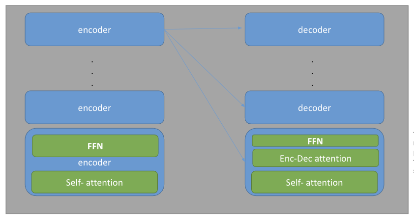
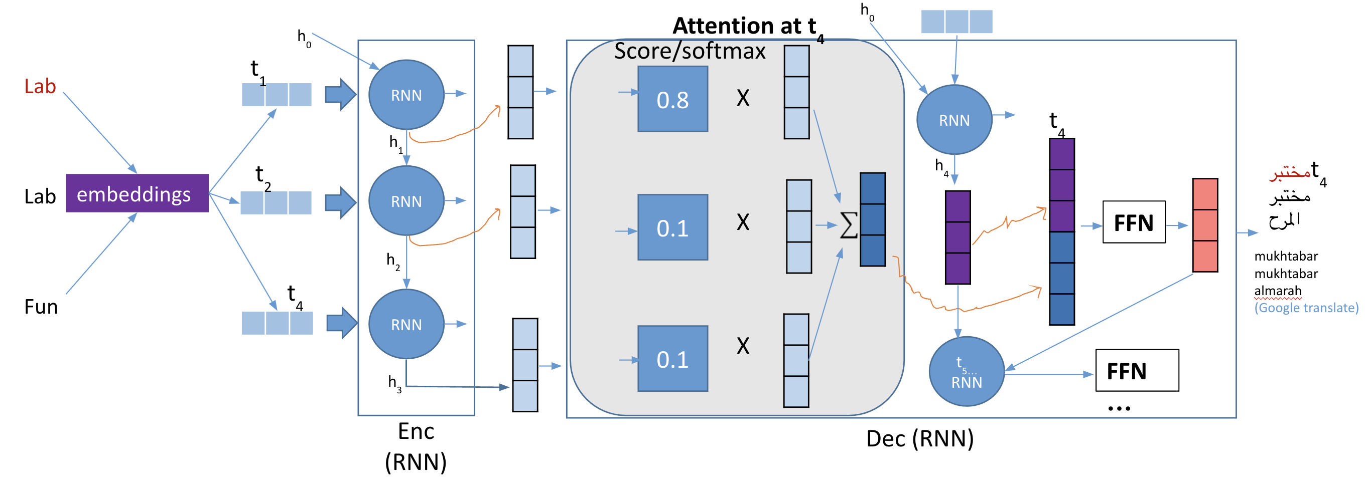
BERT uses Encoder and Decoder architecture. BERT uses multi-layer bidirectional Transformers and encoders. The Encoder is an architecture of connected RNNs. It encapsulates information for all input elements to help the decoder make accurate predictions. The encoder provides the hidden state of the last node (RNNs) to the decoder. This vector encapsulates information for all input elements in order to help the decoder make accurate predictions. Typically machine translation models use RNN as the model base of encoder-decoder architecture. Since this architecture creates a bottleneck of information flow (compressing the contents of the source sequence into a fixed-size vector), Google uses Attention-based Transformer model instead of the traditional RNN architecture. The model can work in parallel, so training is fast and improves translation performance. The attention mechanism consists of the hidden states of all the RNNs, and not just the hidden layer of the last RNN, thus allowing the decoder to look at all of the source sequence hidden state. The model also gives weights (importance) for each hidden state as an additional input to the decoder. Hence, the model selects the context that best fits the current node. Transformers use the encoder-decoder architecture. The internal structure of each encoder and decoder is as follows. The Encoder consists of: 1) a self-attention layer, and 2) a feedforward neural network. Similarly to the encoder, the Decoder also contains the two-layer network with an attention layer in the middle of the two layers.

Transformer Strucutre

The encoder look at other words in the input sentence while encoding a word. The decoder focuses on relevant parts of the input sentence.

Encoder (Enc) - The Final Hidden State of the Encoder

• Encapsulates information for all input elements

• Helps the decoder make accurate predictions

• The encoder provides the hidden state of all nodes to the decoder (not just the hidden state of the last node of the encoder)

Decoder (Dec)

• Selects the hidden state that best matches the current position

  • Calculates the score of each hidden state + softmax

• It then multiples each hidden state by its softmaxed score.

Code Examples are available here: https://colab.research.google.com/drive/1okiRjd5RmulrYXClh0drDhwZvFSGbz1V#scrollTo=BzWBJDqt6FsG

Problem - bottleneck of the Seq2Seq models (e.g Machine Translation)

• Needs to compress the contents of the source sequence into a fixed-size vector

Consider the visual representaiton of this process:

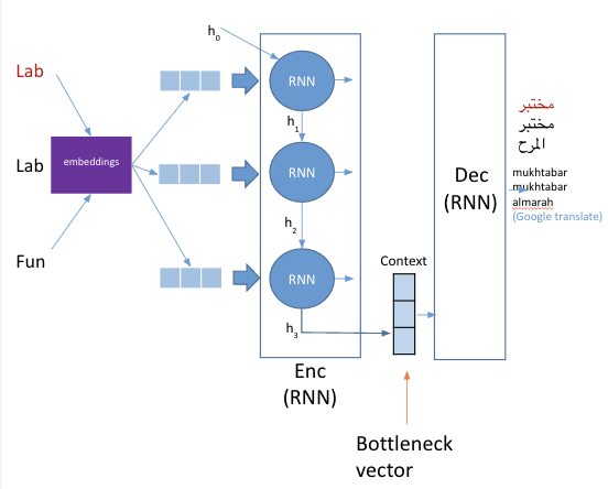
Solution - Attention

• Allows the decoder to look back at all hidden states.

• Give each hidden states a score.

• Multiply each hidden states by its softmaxed score.

Here is an example of the selective attention test: https://www.youtube.com/watch?v=vJG698U2Mvo.

Examples

EnrichrBot

• @BotEnrichr on Twitter - https://twitter.com/BotEnrichr/

• Fine-tuning BERT on a downstream classifcation task

  • Tweets: Gene related / Not

Experiental Learning

• Text Mining Practicum