Chapter 12 - Enrichment Analysis
Contents
Chapter 12 - Enrichment Analysis#
Authors: Sherry Xie
Maintainers: Sherry Xie
Version: 0.1
License: CC-BY-NC-SA 4.0
Introduction#
Background#
Different types of omics studies often generate ranked and unranked gene sets as output. For example:
Gene and protein expression profiling → gene signatures, up/down gene lists
GWAS studies → genes associated with a trait
ChIP-seq studies → gene targets of transcription factors
Identifying common functions for genes in the same set can help explain the molecular mechanisms behind the physiological and pathophysiological changes under investigation. As a practical example, finding connections between a set of genes obtained from a profiling study on a cancer cell line could shed light on what processes seem to drive the disease. That information, in turn, could then further the development or repurposing of drugs to target those disease processes.
Gene sets#
A gene set is a single list of related genes that are usually output by some type of profiling assay.
A gene set library is a collection of several gene sets that are all related to a specific theme or concept. They are commonly stored in the form of Gene Matrix Transposed (GMT) files, which are tab-delimited files with the following format (where \t represents a tab space):
TERM1\tDESCRIPTION\tGENE\tGENE\tGENE\tGENE\tGENE...
TERM2\tDESCRIPTION\tGENE\tGENE\tGENE\tGENE\tGENE...
...
Each line represents a single gene set, where the first term TERM is some annotation or label for the gene set, the second term DESCRIPTION is an optional more detailed description of the gene set, and all following terms are GENES in the set. Gene sets within one library do not have to be the same length.
Enrichment/pathway analysis#
By definition, enrichment analysis is a method for identifying functional or biological terms that are over-represented in a set of genes; while the process can also be performed on other small molecules such as drugs or metabolites, this lecture will primarily focus on genes. Pathway analysis is similar to enrichment analysis, but specifically focuses on identifying biological pathways whose member genes are significantly over-represented in a gene set. Examining sets of genes, rather than individual genes, can reduce noise and lead to more meaningful, robust, and biologically relevant results.
There are a few key steps to enrichment analysis:
Obtain a gene set of interest (ranked or unranked).
Compare the input gene list against a background of gene set libraries. The background determines which genes should actually be used in the analysis, with the default being all genes in the input gene list.
Identify gene sets from the gene set library where genes from the input gene set are over-represented, or enriched.
Enrichment analysis can thus highlight biological themes related to the input gene set, such as:
What biological processes appear to be disrupted?
What cell or tissue types are represented?
Which gene and protein expression regulators are implicated?
“Overrepresentation” vs. “overlap”#
While overlap works in simple cases of gene set comparison, if two gene sets that are very large are compared, the overlap will appear artificially high. Additionally, some genes may be common to many gene sets, and would be less biologically relevant than more unique genes depending on the research question. Consider the following scenario:
Input Gene Set (length 100 genes) & Gene Set A (length 1000 genes): 20 genes overlap

Input Gene Set (length 100 genes) & Gene Set B (length 10 genes): 9 genes overlap
Based on purely overlap, it would appear that Gene Set A is more enriched for the input gene set (20 > 9). However, Gene Set B may actually be more interesting to the researcher, because we can see that 9/10 (90%) genes in Set B are present in the input gene set, while only 20/1000 (2%) from Set A are present. In general, simple overlap tends to produce biased results towards longer gene lists, which is why most enrichment analysis algorithms tend to focus on overrepresentation instead.
Different algorithms for performing enrichment analysis#
Gene set enrichment analysis (GSEA): A well-known algorithm for identifying pathways or functional modules that are enriched for a ranked list of input genes (Subramanian et al., 2005). See the section on GSEA for more information.
Jaccard coefficient: Computes the intersection of two gene sets divided by the union of two gene sets.
Fisher’s exact test: Determines whether two categorical variables are related, e.g. whether an input gene set is related to a particular functional term. See the section on Fisher’s exact test for more information.
Network-based enrichment analysis: A method of identifying significant relationships between gene sets by applying a random walk to a known protein-protein interaction network. (Liu & Ruan, 2013)
Resources for performing enrichment analysis#
GSEA: Gene Set Enrichment Analysis (Subramanian et al., 2005)
DAVID: Database for Annotation, Visualization, and Integrated Discovery (Sherman et al., 2022)
GSEA#
Background#
The Gene Set Enrichment Analysis (GSEA) algorithm (Subramanian et al., 2005) is a method that determines if a ranked list of input genes is significantly associated with some biological function represented by a known gene set. The algorithm is available as an online tool and as a downloadable desktop software.
GSEA algorithm steps#
While the full details of the GSEA algorithm can be found in the publication by Subramanian et al. (2005), a simplified version of the process is detailed below.
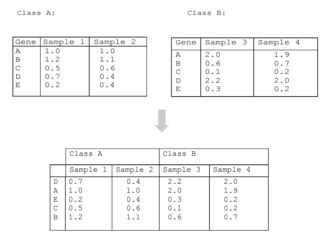
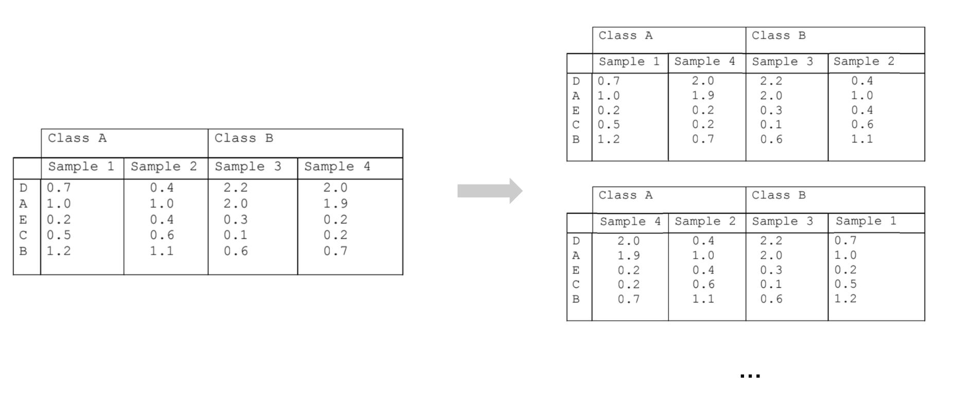
Given gene expression profiling samples from two different conditions, rank the genes by differential expression between samples from the two conditions. In the example figure below, we have two samples each from two conditions, Class A and Class B. In the combined table, the genes are ranked according to their differential expression between the two conditions. Gene D is ranked first because it is most positively differentially expressed in Class B compared to Class A; Gene B is ranked last because it is most negatively expressed in Class B compared to Class A.
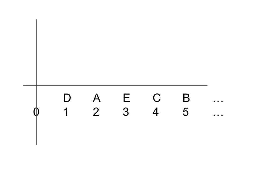
Place the sorted gene ranks along the x-axis of a graph. In the example figure below, the genes from the table above are placed along the x-axis according to their differential expression rank, with Gene D at position 1.
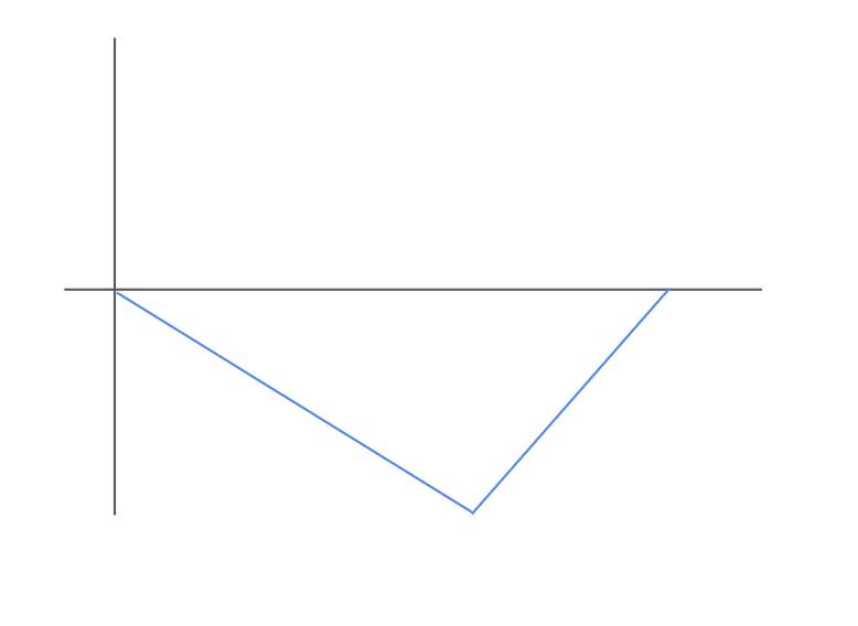
Compare the ranked list to an annotated gene set of interest by computing a running sum, also called a Brownian bridge random walk. In our example, let’s say we are interested in whether the gene set
{B, C}, representing some biological function, is enriched in our gene expression data. Starting from (0,0), we can then “walk” down the ranked genes on the x-axis, and check whether each gene is present in the gene set{B, C}.If the gene at a given position IS NOT in the gene set, we increment by \(-\sqrt{\frac{G}{N-G}}\)
If the gene at a given position IS in the gene set, we increment by \(\sqrt{\frac{G}{N-G}}\) For our example, in which Genes
D,A,Eare not in the gene set, butBandAare, we obtain the following graph:
The supremum of the Brownian bridge plot is the enrichment score (ES). While the supremum may be positive or negative, in this example, we can see that the supremum is negative.
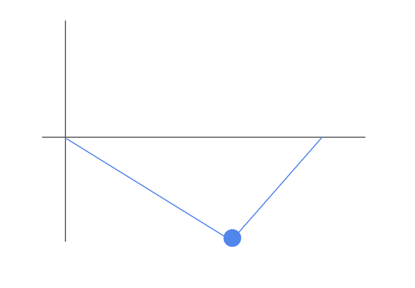
A POSITIVE supremum/ES would indicate that the genes in the comparison set
{B, C}are up-regulated in Class B compared to Class A.A NEGATIVE supremum/ES would indicate that the genes in the comparison set
{B, C}are down-regulated in Class B compared to Class A.A lack of significant deviation from y = 0 indicates the genes in the comparison set do not appear to be significantly differentially expressed between the two conditions. Note that the interpretation of the ES depends on the data being examined; in the cases of gene expression data from GWAS or ChIP-seq studies, a positive ES will be more relevant because we are generally only interested in genes with positive associations.
Estimate the significance of the relationship between the rank list and the annotated gene set. To compute the significance of the ES, the algorithm essentially will swap the class labels of the samples many, many times and repeat the above steps to compute the ES for all swapped comparisons.
The significance value can then be calculated from the number of instances in which the randomly swapped ES is closer to 0 than the actual ES.
For a more detailed overview of the process, including example Brownian bridge plots for gene expression comparisons with expected outcomes, please refer to Subramanian et al. (2005).
Fisher’s Exact Test#
Background#
Fisher’s Exact Test (FET), named after its creator Ronald Fisher, is a statistical test to determine if there is a significant relationship between two or more categorical variables, and is a common approach for quantifying over-representation between sets. For a given gene set obtained from transcriptomics profiling data, FET can identify if the input genes are over-represented in annotated gene sets that reflect prior knowledge.
Fisher’s Exact Test is well known as the statistical test used in the “lady tasting tea” experiment from Fisher’s 1935 book The Design of Experiments, which examined whether or not the mentioned lady, Muriel Bristol, could actually identify whether tea or milk was added first to a cup based solely on taste.
Contingency tables#
In the simplest version of FET, which examines the association between two categorical variables, the test can be visualized using a contingency table. An example table is shown below, adapted from Wikipedia.
Category X |
Category Y |
Total |
|
|---|---|---|---|
Trait 1 |
a |
b |
a + b |
Trait 2 |
c |
d |
c + d |
Total |
a + c |
b + d |
a + b + c + d (=n) |
In the table, a, b, c, d each represent the number of observations that belong to a specific category and trait pairing. For instance, b indicates how many observations in Category Y also have Trait 1.
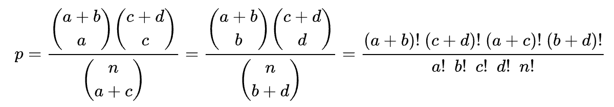
General FET formula#
From the contingency table above, we can derive a formula for computing the probability of observing a given table of values (out of all possible table values). We make this computation under two key assumptions about the data:
There is no association between the two categories. This is also the null hypothesis.
The marginal values, i.e. the row and column totals, are fixed. The total number of observations for each category remain the same across all possible tables.
The formula for the probability p is as follows:
Gene expression example#
The table below gives an example contingency table that represents some data from a gene expression study, with all numbers chosen for simplicity. In this example, the study measured the expression of 10,000 different genes under perturbation by a drug, and the researchers were able to generate a differential gene expression signature from the results. They now want to identify whether or not the differentially expressed genes are enriched for a specific biological pathway. If the genes that have their expression disrupted by the drug are disproportionately represented in the gene set corresponding to the pathway, that could be an indication that the tested drug has an affect on the pathway.
Differentially expressed |
Not differentially expressed |
Total genes |
|
|---|---|---|---|
In pathway gene set |
80 |
200 |
280 |
Not in pathway gene set |
20 |
9700 |
9720 |
Total genes |
100 |
9900 |
10000 |
From the example table above for gene expression results, perhaps you could argue just by eye that there is some association between the drug and the pathway, since the table shows that 80 out of 100 differentially expressed genes appear to belong to the pathway of interest (80%). However, what if only 50 out of 100 differentially expressed genes were in the comparison pathway set? There needs to be a systematic method to quantify the degree of relatedness between the differentially expressed genes and the pathway.
Before discussing the specifics of Fisher’s exact test, it may be useful to first discuss some alternative methods.
Simple overlap vs. FET#
In the section on Overrepresentation vs. Overlap above, we saw how simple overlap may not effectively capture the relationship between gene sets of different size. We can demonstrate that principle again here using the gene expression example.
In the example table above, we have:
100 differentially expressed genes in the drug perturbational signature
280 genes in the pathway associated gene set
80 overlapping genes between the above two gene sets
Based on these numbers alone, it is difficult to definitively state whether or not the genes from the signature are enriched for the pathway, as there is nothing to compare to the value of “80”. This makes it difficult to determine the degree of enrichment.
Furthermore, consider if the researchers simultaneously also looked at a second pathway gene set:
100 differentially expressed genes in the drug perturbational signature
560 genes in the second pathway associated gene set
81 overlapping genes between the above two gene sets
If we were only using overlap to quantify enrichment, it would be tempting to say that the differentially expressed genes are more enriched for the second pathway because 81 > 80 – but that fails to take into account that there are many more genes in the second pathway gene set that do NOT overlap (479) than there are in the original pathway gene set (20). Because the sizes of the gene sets are so different, simply comparing the overlap could lead to an inaccurate interpretation of the results.
Jaccard index vs. FET#
The Jaccard index is another statistic that can be used to compare sets, and is generally defined as the ratio intersection:union, referring to the set theory definitions of the intersection and union. The Jaccard index evaluates the overlap between two sets (intersection), but additionally considers the combined size of both sets (union).
In the gene expression above, the Jaccard index J(Differentially Expressed, Pathway) would be computed as follows:
\( J = \frac{80}{(100+280)-80} \approx 0.267 \)
where the numerator represents the intersection (80), and the denominator represents the union between the set of differentially expressed genes and pathway genes (100 + 280, minus the 80 overlapping genes).
Although we can now account for the size of the gene sets, it is still possible for the results to be skewed. Imagine that instead of there being 100 differentially expressed genes and 280 pathway genes, there are instead 80 total differentially expressed genes and 300 pathway genes, and we still observed 80 genes overlapping between the two sets. The computation of the Jaccard index would result in the same numerical value as above:
\( J = \frac{80}{(80+300)-80} \approx 0.267 \)
However, the context has now changed from the original scenario – every single one of the differentially expressed genes now appears to belong to the pathway, which could make an even stronger argument that the drug which led to the gene signature affects the given pathway. But that potentially significant difference in meaning is not reflected in the numerical results.
Applying FET to gene expression#
Now that we have gone over two alternative methods and their strengths and flaws, we can see how Fisher’s Exact Test might address those shortcomings.
Before performing any computations, the two assumptions required for FET can be reframed in the context of the example as well:
The null hypothesis is that the pathway of interest is not overrepresented among the differentially expressed genes in the drug perturbational signature.
Of the 10000 total genes, 9900 of the genes are not differentially expressed in the signature, and 9720 of the genes are not associated with the pathway.
We can then examine all possible configurations of the contingency table, with a few examples shown below.
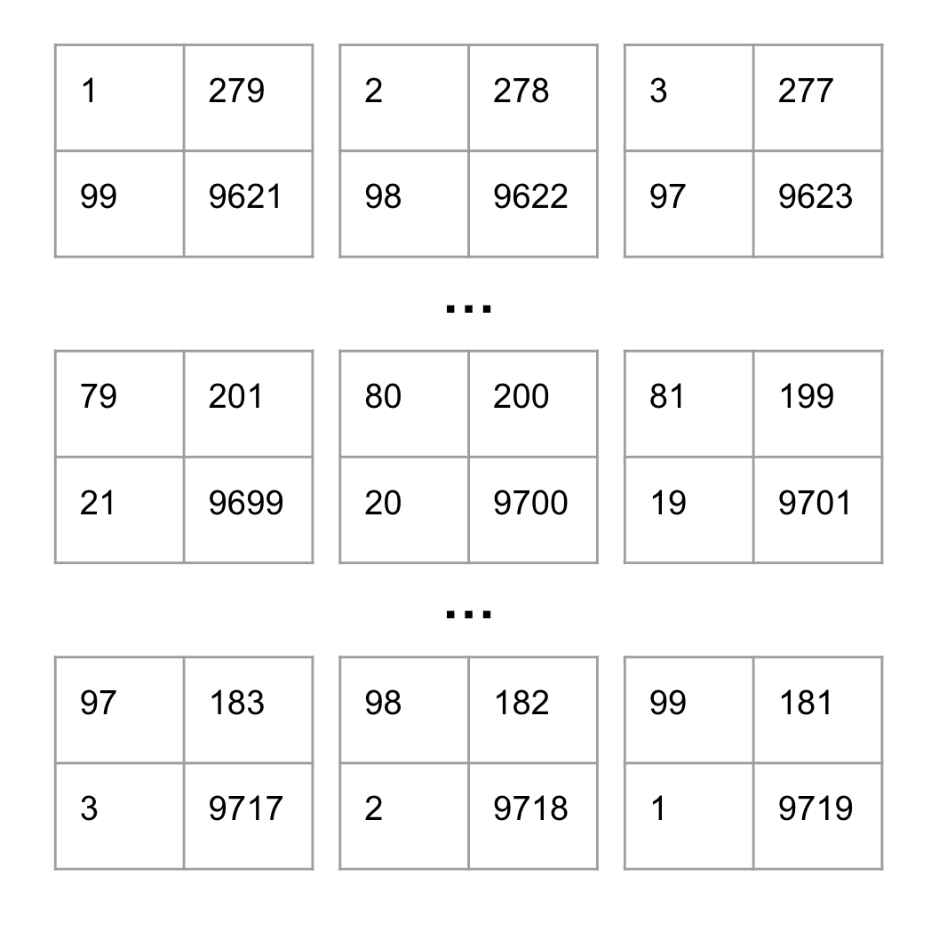
Note that each contingency table occurs with a different likelihood. For instance, consider how many ways a single gene could be both differentially expressed AND in the pathway gene set, compared to how many different pairs of genes could be both differentially expressed AND in the pathway gene set.
With all of the contingency table possibilities mapped out, we can then compute the probability of obtaining the observed table by counting how many ways there are to select without replacement…
80 differentially expressed genes out of 280 belonging to the pathway gene set?
20 differentially expressed genes out of 9720 NOT belonging to the pathway gene set?
100 differentially expressed genes out of 10000 total genes? If we plug the observed values from our contingency table into the formula from above, we obtain the following probability for our observed values: (280 choose 80) x (9720 choose 20) / (10000 choose 100) = 1.04e-109
As we can see from the process above, Fisher’s exact test takes into account the size of both gene sets being compared, as well as the total number of genes in the comparison pool, in order to provide a potentially more nuanced metric for enrichment than simple overlap and the Jaccard index.
Significance of FET#
In the example above, we obtained a numerically low probability of getting our observed results, which seems to suggest that the two categories under study are indeed related – in other words, that the drug perturbation seems to affect the expression of genes in the given pathway of interest. However, it may be useful for many researchers to have a more systematic method for computing the significance of the results, especially in the context of enrichment analysis.
This is where the concept of a hypothesis test, which has been alluded to throughout this tutorial, comes into relevance. Earlier, one of the assumptions made was the null hypothesis, which is the hypothesis that there is no association between the two categories under study. The null hypothesis may not be proved, but may be disproved based on observed results in favor of an alternative hypothesis. For Fisher’s exact test, the alternative hypothesis generally is the hypothesis that there is an association between the two categories at hand. In general, the “significance” of a given result simply refers to how likely it is to see that result under the circumstances where the null hypothesis is true.
For the gene expression example detailed above, we can rephrase the question to “How likely is it to observe results at least as extreme as what was observed, if there is truly no relationship between the drug and the pathway?” Another way of thinking about it is “How likely is it to observe a result that occurs with probability at most 1.04e-109, out of all possible results?”
This hypothesis test is generally referred to as a one-sided hypothesis test. The key here is to understand that while the formula above already computed the probability of observing a single table, the significance test is interested in the probability of observing that table along with the probabilities of observing any table demonstrating a greater association between the drug and the pathway:
Probability of obtaining exactly 80 genes that are differentially expressed AND in the gene set (what we already computed earlier)
Probability of obtaining > 80 genes that are differentially expressed AND in the gene set
Summing together these probabilities will result in the significance value for the results.
A note on two-sided hypothesis tests: As the name suggests, the two-sided significance value can be computed by summing the probabilities for all possibilities with probability less than or equal to the observed results. This will often roughly be double the one-sided significance value, but not always exactly.
Key Terms#
Gene set: A collection of unique genes that are somehow related, and usually obtained as a result of an omics profiling study.
Background: The set of actual genes to be considered for comparison in any enrichment analysis study. Typically, all genes in the input set are used for comparison, but there is a chance this may bias the results towards terms that describe the original sample from which the input genes were extracted, rather than terms relevant to the condition being studied.
Gene set library: A set of related functional terms, each associated with a set of genes based on prior knowledge.
Enrichment analysis: Examining the overrepresentation or “enrichment” of genes associated with specific functional terms in a given gene set.
Pathway analysis: Examining the overrepresentation or “enrichment” of genes associated with specific biological pathways in a given gene set.
References#
Subramanian A, Tamayo P, Mootha VK, Mukherjee S, Ebert BL, Gillette MA, Paulovich A, Pomeroy SL, Golub TR, Lander ES, Mesirov JP. Gene set enrichment analysis: a knowledge-based approach for interpreting genome-wide expression profiles. Proc Natl Acad Sci U S A. 2005 Oct 25;102(43):15545-50. doi: 10.1073/pnas.0506580102. Epub 2005 Sep 30. PMID: 16199517; PMCID: PMC1239896.
Liu L, Ruan J. Network-based Pathway Enrichment Analysis. Proceedings (IEEE Int Conf Bioinformatics Biomed). 2013:218-221. doi: 10.1109/BIBM.2013.6732493. PMID: 25327472; PMCID: PMC4197800.
Kuleshov MV, Jones MR, Rouillard AD, Fernandez NF, Duan Q, Wang Z, Koplev S, Jenkins SL, Jagodnik KM, Lachmann A, McDermott MG, Monteiro CD, Gundersen GW, Ma’ayan A. Enrichr: a comprehensive gene set enrichment analysis web server 2016 update. Nucleic Acids Res. 2016 Jul 8;44(W1):W90-7. doi: 10.1093/nar/gkw377. Epub 2016 May 3. PMID: 27141961; PMCID: PMC4987924.
Sherman BT, Hao M, Qiu J, Jiao X, Baseler MW, Lane HC, Imamichi T, Chang W. DAVID: a web server for functional enrichment analysis and functional annotation of gene lists (2021 update). Nucleic Acids Res. 2022 Mar 23;50(W1):W216–21. doi: 10.1093/nar/gkac194. Epub ahead of print. PMID: 35325185; PMCID: PMC9252805.
Mi H, Muruganujan A, Huang X, Ebert D, Mills C, Guo X, Thomas PD. Protocol Update for large-scale genome and gene function analysis with the PANTHER classification system (v.14.0). Nat Protoc. 2019 Mar;14(3):703-721. doi: 10.1038/s41596-019-0128-8. Epub 2019 Feb 25. PMID: 30804569; PMCID: PMC6519457.
Fisher, RA. On the Interpretation of X squared from Contingency Tables, and the Calculation of P. Journal of the Royal Statistical Society. 1922;85(1):87-94. doi: 10.2307/2340521.
Wikipedia contributors. Jaccard index. Wikipedia, The Free Encyclopedia. October 6, 2022. Available at https://en.wikipedia.org/wiki/Jaccard_index.
Wikipedia contributors. Fisher’s exact test. Wikipedia, The Free Encyclopedia. October 22, 2022. Available at https://en.wikipedia.org/wiki/Fisher%27s_exact_test.