Chapter 16.2a - Introduction to Deep Learning
Contents
Chapter 16.2a - Introduction to Deep Learning#
Authors: Daniel J. B. Clarke
Maintainers: Daniel J. B. Clarke
Version: 0.1
License: CC-BY-NC-SA 4.0
Prerequisites#
Please ensure you’ve first completed Introduction to Machine Learning.
Recap
Definitions & Terminology including
AI, ML, Deep Learning
Supervised, Unsupervised, Semi-supervised, Reinforcement Learning
Regression; Binary, Multi-class, Multi-label Classification
Various classes of models
Linear Models
Dimensionality Reduction
Clustering
Decision Trees
ML In Practice
Normalization
Regression, Classification Metrics
Cross Validation
Scikit-Learn

Background#
What is “Deep” Learning?#
Deep learning refers to ML with extremely high number of parameters typically tuned (or learned) by gradient descent on lots of data. Examples of Deep Learning Models include:
Alpha Zero - Super-human Shogi, Chess, and GO
GPT-3 - Large Language Model
Alpha Fold - Protein Structure Prediction
DALL-E 2 - Text to Image
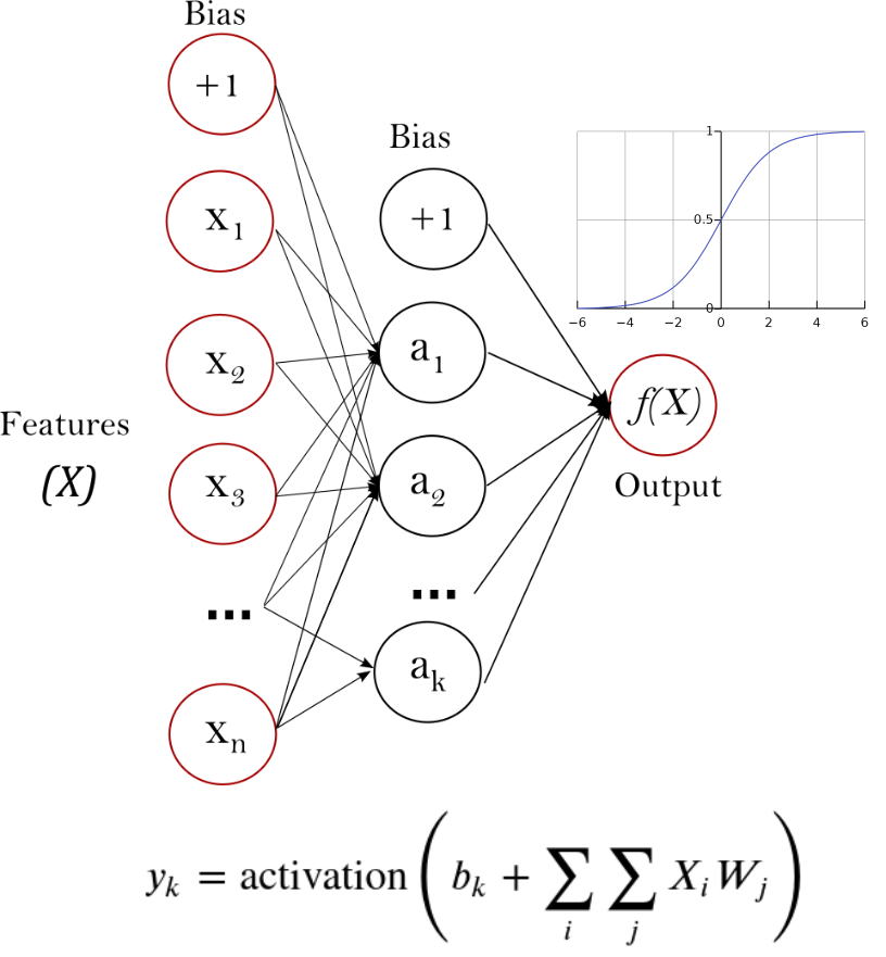
Feed Forward Neural Network (FFNN)#
An architecture which facilitates weighted summations of sample features to directly compute a desired output. Parameters are tuned to minimize error via gradient descent using a technique called back propagation to support a highly flexible architecture.
Different activation functions & regularizations & number of layers can be applied.
Explore the effect that the architecture has on performance: https://playground.tensorflow.org/
Gradient Descent & Back Propagation#
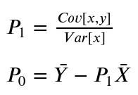
Classic algorithms often had different mathematical techniques to optimize few parameters.
For example, ordinary least squares(linear models) uses
Neural networks use auto differentiation (AD) to build a computational graph of gradients to support practically any finite architecture (Fig A). Gradient descent algorithms then are used to numerically optimize parameters, notable methods & animation of this process shown in Fig B.


Embeddings#
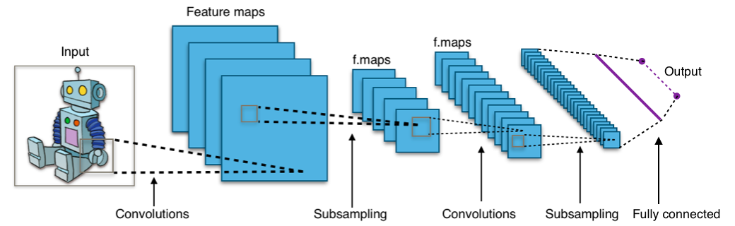
Convolutional Neural Network (CNN)#
CNNs connects spatially co-located dimensions in the input vector, whereas the alternative is to assume all dimensions are completely independent. CNNs offer several advantages to dense networks in certain types of data like image & time series.
Example mainstream CNNs include: ImageNet, Residual Net (ResNet), & Inception
Word2Vec#
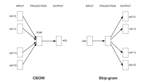
Word2Vec described two ways to get efficient vector representations of words whereas the alternative is to represent each word as a one-hot-encoded vector the size of the dictionary.
CBOW walks through the sentence predicting the middle word (Fig A).
Skip-Gram tries to predict the words next to a given word (Fig B).
The inside of these models can be used to assign a vector to a given word, these vectors have unique properties making them useful for downstream tasks (Fig C).
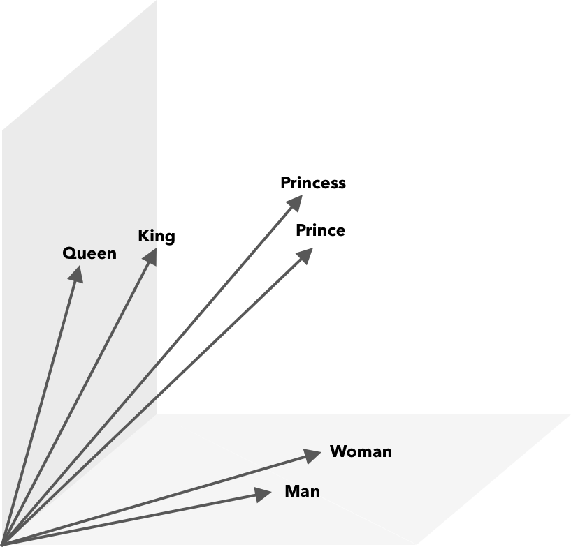
King - Man + Woman = Queen
Architectures#
Autoencoder Networks#
A neural network variant which trains a neural network to recover the original data through a bottleneck layer of lower dimensionality. Behaves as a more flexible & non-linear, though less interpretable PCA alternative.
Variations on this of note include:
Denoising Autoencoder: input is corrupted to provide training data diversity make the code more robust.
Variational Autoencoder (VAE): probability distribution used for the code.
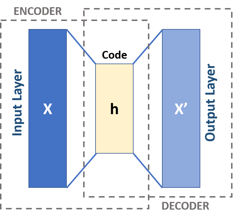
Minimize difference between X & X’
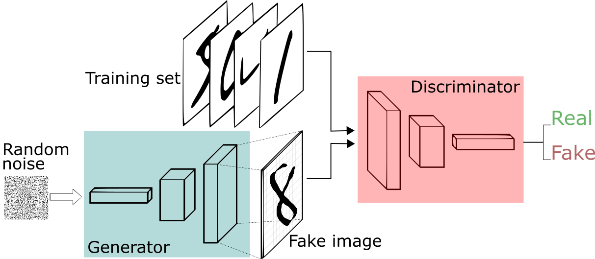
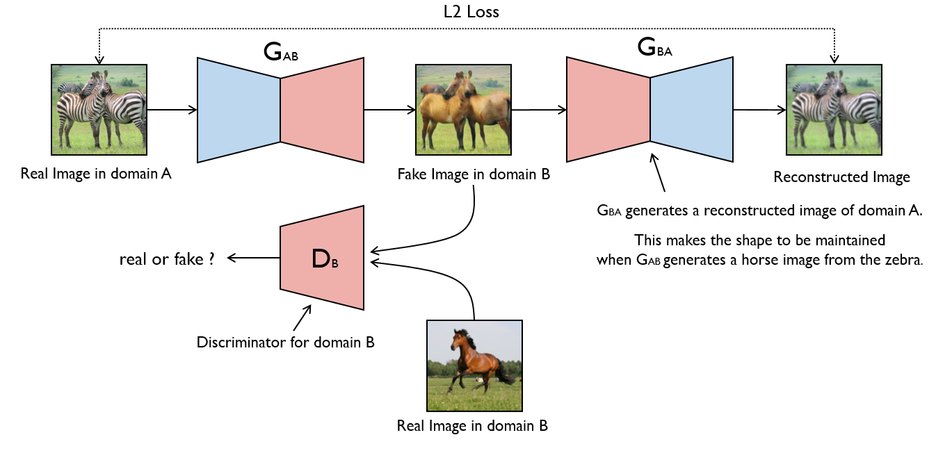
Generative Adversarial Networks (GAN)#
A neural network “generator” which learns to produce “fake” samples, and a neural network “discriminator” which learns to distinguish “fake” samples from real ones, jointly trained.
Variants of note include:
Conditional GAN: Condition the generator for directing new sample creation.
CycleGAN: Unpaired translation between two independent data types with unlabeled data (Fig B).
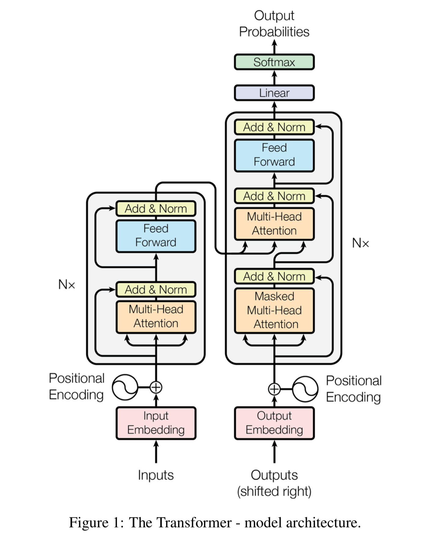
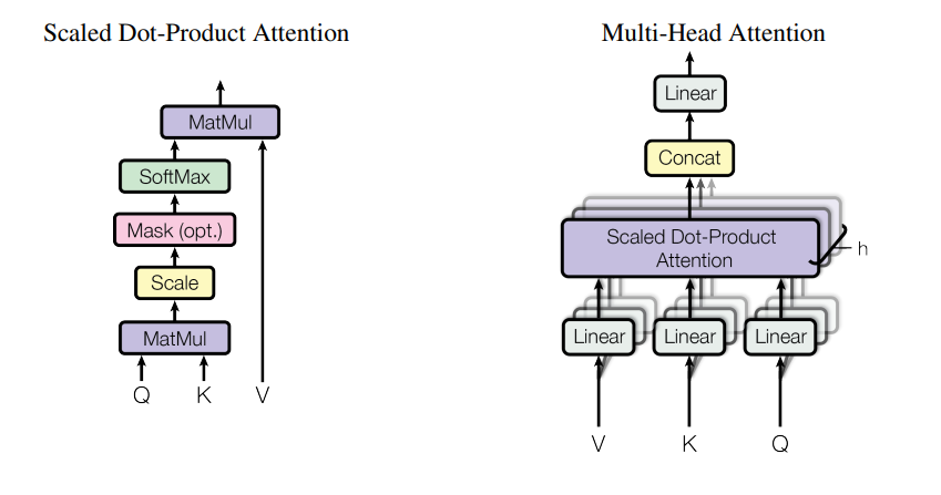
Attention & Transformers#
Attention allows a network to assign a mask to input layer, letting it focus on specific subsets (Fig A). This can be stacked several times (Fig B). The Transformer architecture uses these along FFNNs and residual connections to achieve state of the art on NLP tasks (Fig C).
Transformers are also applicable to other data modalities.
Deep Learning in Practice#
Under/Over Fitting#
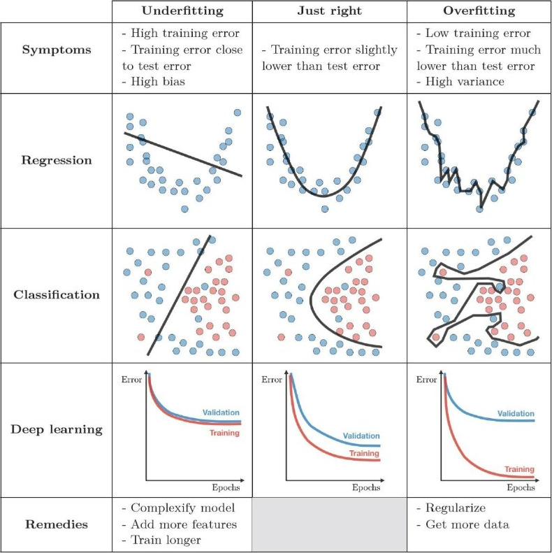
Given the massive number of parameters in Deep Learning, it is very possible for the model to overfit–fitting too well such that generalization suffers.
Under fitting is also possible, the network will sometimes just produce the average.
These situations can be addressed by tuning the model architecture, or addressing problems with data normalization.
Loss & Activation Cheat Sheet#
This requires a lot of math to explain so here I just provide a cheat-sheet & some ”sane” first choices; it will take some research when these don’t work well
For Hidden layers: __ __ activation=relu
For Output layers:
Regression: activation=linear, loss=mse
Classification:
Binary: activation=sigmoid, loss=binary_crossentropy
Multi-Label: activation=sigmoid, loss=binary_crossentropy
Multi-Class: activation=softmax, loss=categorical_crossentropy
Python Libraries#
Both TensorFlow & PyTorch are very popular and continue to be developed. At the time of writing, the choice is mostly preference since both are equally capable of being tweaked and deployed in production.
__TensorFlow: __ An end-to-end machine learning platform.
Open Source software, made mostly by Google
Standard algorithms can often be done in less code than PyTorch at the cost of making non-standard usage slightly more complicated.
PyTorch : A machine-learning framework.
Open Source software, made initially by Meta AI
Slightly more usage in the research community, often more pythonic than tensorflow. A bit “lower level” in the sense that certain things like applying gradients are more explicit in PyTorch.


Conclusions#
In this lecture we learned about:
Models
FFNN
Autoencoders
GANs
Transformers
Embeddings
CNN
Word2Vec
Attention
Practical Concepts
Gradient Descent & Back Propagation
Under/Over Fitting
Loss & Activation Functions
Deep Learning Libraries
Experiential Learning#
Deep Learning Practicum