Working with high dimensional data

High Dimensional Data

High-dimensional data is data that has a large number of dimensions, or variables. This can make it difficult to work with, visualize, and understand the data. Some examples of high-dimensional data include gene expression data, images with many pixels, and text data with many words or documents.

• Gene expression data is a type of high-dimensional data that measures the levels of expression of many genes in a sample. A single gene expression profile contains quantifications for thousands of genes. This data can be used to understand how different genes are related to each other and to different biological processes.

Gene expression is an example of high dimensional data with thousands of genes as the dimensions.

• Images with many pixels are another example of high-dimensional data. For example, a high-resolution digital photograph can have millions of pixels, each of which has three color channels (red, green, and blue).

• Text data with many words or documents is also an example of high-dimensional data. For example, a corpus of text data that includes thousands of documents can have many dimensions, such as the words used in each document and the frequency with which they appear.

Curse of high dimensionality

The curse of dimensionality refers to the challenges that arise when working with high-dimensional data. In high-dimensional space, the volume of the space increases exponentially with the number of dimensions. This can lead to issues such as the need for a large amount of data to adequately represent the space, and the difficulty of visualizing and understanding the data. Additionally, many machine learning algorithms are not well suited to working with high-dimensional data, which can make it difficult to extract useful insights from it.

High dimensional data poses a challenge for machine learning because it can lead to decreased model performance due to the difficulty in modeling and analyzing the large number of dimensions, as well as the decreased relevance of each individual feature.

In high-dimensional space, the volume of the space increases much faster than the surface area. To understand why, imagine a unit cube in three-dimensional space. If you increase the length of each side by a factor of two, the surface area of the cube will increase by a factor of four, while the volume will increase by a factor of eight. In higher dimensions, the gap between the increase in surface area and the increase in volume becomes even greater. For example, in ten-dimensional space, if you increase each side of a unit hypercube by a factor of two, the surface area will increase by a factor of 1024, while the volume will increase by a factor of 2048. This means that as the number of dimensions increases, the volume of the space grows much faster than the surface area.

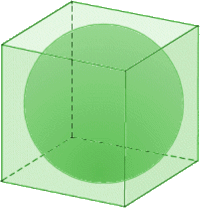
Hypershpere and Hypercube Volume

As a result points will be more likely located on the outer shell of the volume the more dimensions there are. This can also be visualized by comparing the volume of a hypercube and a hypersphere.

Volume of

• Hypersphere:

\[ V_{sphere}(d,r) = {2r^{d} \pi^{d/2} \over {d \Gamma(d/2)}} \]

\[ \Gamma(n) = (n-1)! \]

• Hypercube:

\[ V_{cube}(d,r) = (2r)^{d} \]

Example

Let’s look at an example for different numbers of dimensions

\( d=2 \) (area of a circle)
\( r=1 \)

\( V_{sphere}(2,1) = {2 \pi^{2/2} \over {2 \Gamma(1)}} = \pi \)
\( V_{cube}(2,1) = 2^{2} = 4 \)

---

\( d=4 \)
\( r=1 \)

\( V_{sphere}(4,1) = {2 \pi^{4/2} \over {4 \Gamma(2)}} = 2 \pi^{2} / 4 = 4.935 \)
\( V_{cube}(4,1) = 2^{4} = 16 \)

---

\( d=8 \)
\( r=1 \)

\( V_{sphere}(8,1) = {2 \pi^{8/2} \over {8 \Gamma(4)}} = {2 \pi^{4} / 48 \pi } = 4.05 \)
\( V_{cube}(8,1) = 2^{8} = 256 \)

Interestingly the volume of the hypersphere initially increases and then starts shrinking again with increasing number of dimensions.

High dimensional data as shown in the example above does not neccessarily conform to out intuition we gain from lower dimensional data.

Managing high dimensional data

While a large amount of data can be beneficial for machine learning, it is important to manage it properly to avoid overfitting and building models that are not generalizable. This requires careful consideration of how to handle the high dimensional nature of the data in order to achieve the best possible results. There are several techniques that can be helpful:

Naive use of high dimensional data in machine learning can lead to overfitting and bad model performance.

• Feature selection

  • univariate feature selection

  • feature engineering: e.g. SIFT

  • feature importance ranking

  • recursive feature elemination

• Dimensionality transformation

  • principal component analysis (PCA), singular value decomposition (SVD), or t-distributed stochastic neighbor embedding (t-SNE)

• Regularization

  • impose penalty to the machine learning algorithm objective function to reduce number of dimensions

• Ensemble learning

Feature Selection

Feature seelction methods try to focus on dimensions that maximize prediction performance and dismiss dimensions that seem less important.

Univariate Feature Selection

Univariate feature selection will try to find the top dimensions that matches individually the best with the response variable that we try to predict. Depending on the type of prediction (regression/classification) we can use correlation or the chi2 test. The user has to specify a number of dimensions that we want to retain.

from sklearn.datasets import load_iris
from sklearn.feature_selection import SelectKBest
from sklearn.feature_selection import chi2

X, y = load_iris(return_X_y=True)
print("Higher dimension data", X.shape)

X_new = SelectKBest(chi2, k=2).fit_transform(X, y)
print("Lower dimension data", X_new.shape)

Higher dimension data (150, 4)
Lower dimension data (150, 2)

This approach is somewhat naive and ignores the possibility that the dimensions in the data might be dependend on each other.

Feature Importance Ranking

More advanced versions of identifying important features can be imagined. As mentioned before, observing the relationship of a single dimension to the output variable might miss relevant information regarding relationships between variables. A better way to find important features can be achieved with these strategies below:

• Using Decision trees / Random Forests: The feature importance is calculated by the average decrease in impurity over all trees in the forest, weighted by the number of samples that pass through the node. The feature importance is usually generated during the model training step.

from sklearn.ensemble import RandomForestRegressor
from sklearn.datasets import load_iris

X, y = load_iris(return_X_y=True)
rf = RandomForestRegressor(n_estimators=100)
rf.fit(X, y)

print("Feature Importance:", rf.feature_importances_)

Feature Importance: [0.00605688 0.00595046 0.53252666 0.45546599]

As we see in the example above the last two dimensions seem much more important than the first two when predicting the response variable.

Permutation Based Feature Importance

In contrast to Random Forests which can infer the information of feature importance directly from a trained model, other algorithms might not support the same. For example a Support Vector Machine or a Deep Neural network does not directly compute the importance of features. In such a case we can use a method that will basically always work, no matter what the ML algorithm is.

Permutation Based Feature Importance works with all machine learning algorithms.

Warning

The permutation based importance has some drawback to keep in mind:

• when features are highly correlated they might be reported as unimportant

• calculating the permutations can be slow

First we train a model and then the algorithm will apply random permutations on the input features. Permuting important features will result in decreased prediction performance, while the model should be more robust to changes in permutations of less important features.

from sklearn.model_selection import train_test_split
from sklearn.datasets import load_iris
from sklearn.inspection import permutation_importance

from sklearn.svm import SVC

X, y = load_iris(return_X_y=True)
X_train, X_test, y_train, y_test = train_test_split(X, y, test_size=0.25, random_state=12)

clf = SVC(kernel='linear')
res = clf.fit(X_train, y_train)

perm_importance = permutation_importance(clf, X_test, y_test)

print("Feature Importance:", perm_importance.importances_mean)

Feature Importance: [0.03157895 0.01578947 0.55789474 0.17368421]

Recursive Feature Selection

Recursive feature elimination (RFE) is a technique for selecting a subset of relevant features from a larger set of features in a dataset. It works by training an external estimator, such as a linear model, on the initial set of features and using a specific attribute or callable to determine the importance of each feature. The least important features are then removed from the current set of features, and the process is repeated recursively on the reduced set until the desired number of features is reached. This helps to identify and select the most relevant and informative features for the model, while minimizing the risk of overfitting and improving model performance.

In a top down approach features get eliminated one-by-one until the desired number of features/dimensions remains.

from sklearn.datasets import load_iris
from sklearn.inspection import permutation_importance

from sklearn.svm import SVC
from sklearn.feature_selection import RFE

X, y = load_iris(return_X_y=True)

clf = SVC(kernel='linear')

selector = RFE(clf, n_features_to_select=2, step=1)
selector = selector.fit(X, y)
selector.support_

print("Features Selected:", selector.support_)

Features Selected: [False False True True]

Dimensionality Transformation

Dimensionality transformation involves creating new dimensions from existing dimensions in order to better describe the data. This process is predicated on the assumption that the underlying dimensions of the data are fewer in number than the dimensions used to describe it. By combining dimensions in this way, it is possible to more effectively capture the underlying structure of the data and reduce the complexity of the representation.

Data Redundancy